Updated: September 19, 2023
Unlock the Secrets of PriceLabs’ Cutting-Edge Dynamic Pricing Algorithm. Delve into the Depths – A Technical Adventure Awaits!
The document below may get a little technical, but it will help you understand the “black box” of where our Dynamic Pricing recommendations come from. You don’t have to read this to understand how to use PriceLabs, but if you were inclined to learn about algorithms – then strap on!
To help you learn how to use the product – we have daily live onboarding sessions, training videos on YouTube, and a detailed knowledge base to help you use PriceLabs effectively. But if you wanted to get technical and dive into the world of math to understand how the recommendations are calculated – this would be a great read.
Word of caution: This is a technical read with engineering, mathematical concepts, and graphs.
Unlock 1: Data collection
Data: The new oil!
We get information about your property from your property management system or Airbnb / Vrbo if you directly integrate those. This data helps us understand where your listing is located, listing-related details (e.g., bedroom count, how many it sleeps), its future prices, its reservation history, and availability.
Using market data to price your properties is at the core of PriceLabs. We scan various booking portals and direct data sources to build a unified understanding of what’s happening worldwide.
Currently, we scan over 10 million individual units from Airbnb, Vrbo, and Booking.com. In addition, we get direct source data from Key Data to understand actual booking patterns.
You may have likely heard that scrapped data is not clean and thus not good. This is mainly said because scraped data can have owner blocks – so you don’t know if it’s a booking or a block. We apply block removal logic techniques to determine whether a booking on scrapped data is a block or a booking. Some examples include market-wide bans – long bookings with the same start and end date across listings, listing level repeated patterns, price anomalies, etc.
Unlock 2: Hyper-local compset
Neighborhood fetch: Devil lies in the details!
We have found that even listings in the same city can have significantly different market trends depending on their location, resulting in completely different seasonality, day-of-week patterns, and events. Because of this, we focus our modeling on prices on hyper-local data that allow us to capture trends that are potentially unique to a small pocket of listings.
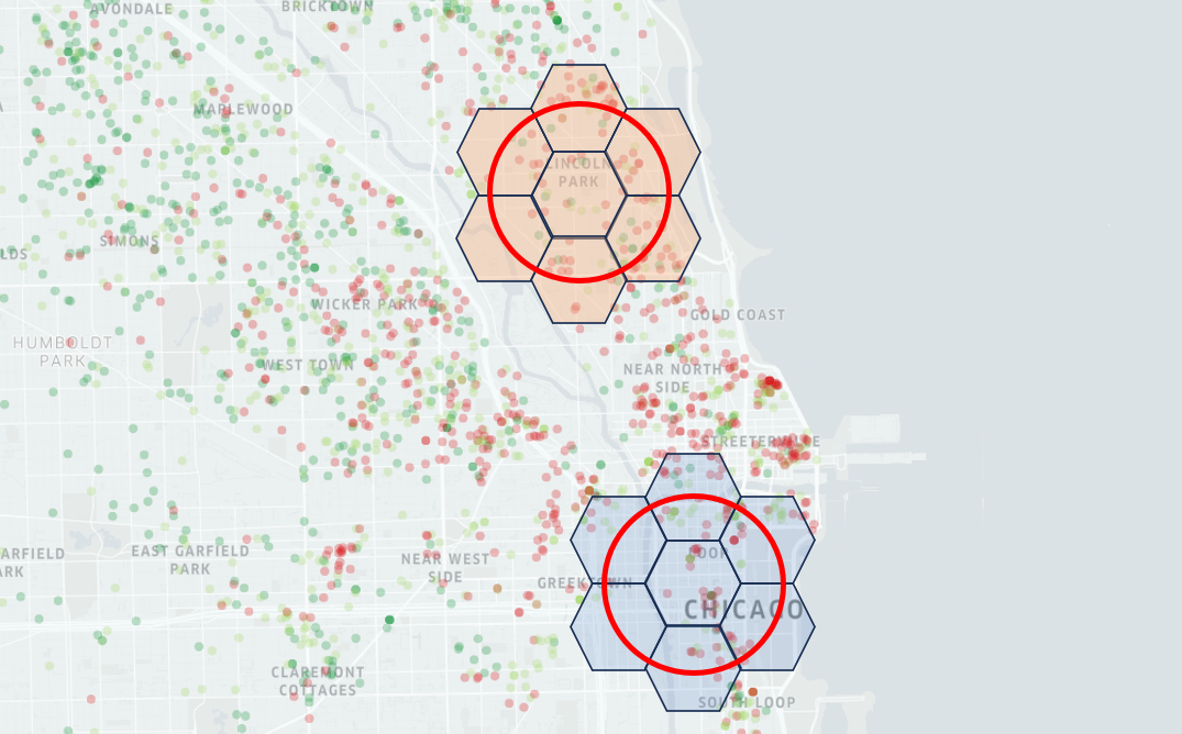
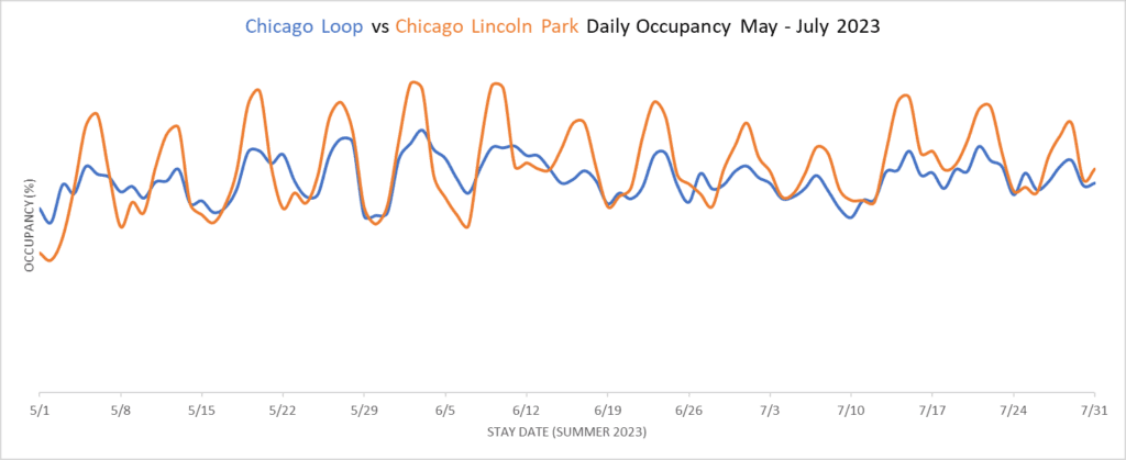
Example: Let’s look at an example of two Chicago neighborhoods: Loop and Lincoln Park. They are only 4 KM (2.5 miles) apart from each other. But when we look at the data, day-of-week patterns for the two neighborhoods are very different. This primarily comes down to Chicago Loop being the business district with stronger mid-week demand from business travelers, while Lincoln Park attracts more tourist demand as there aren’t many offices there.
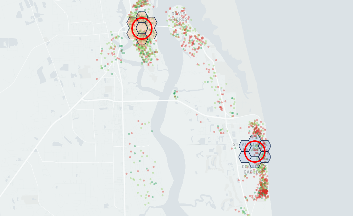
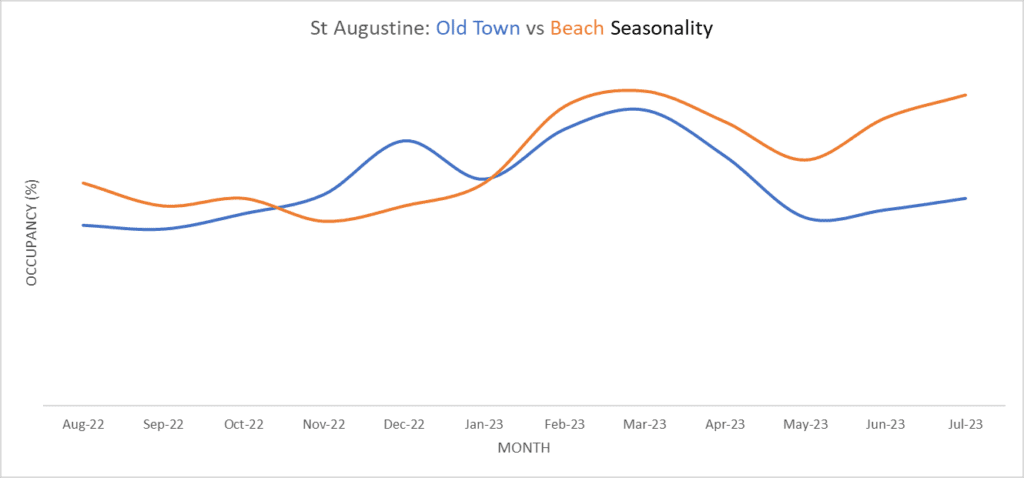
Example: Let’s now look at St. Augustine, FL. This time we are looking at Beach and Old Town. Even though they are only 8 km (5 miles) apart, the seasonality is quite different.
As seen in the chart below, the Old Town area has a Christmas peak while the Beach area has a Summer peak.
The above examples and many others led us down the path of building our new pricing algorithm, Hyper Local Pulse (HLP).
We now look at a hyper-local market on Airbnb or Vrbo to price a specific property. This is defined by 350 similar-sized nearby listings in a maximum radius of 15km – The actual radius is determined dynamically.
From Pedro, Sr. Data Scientist: “At the heart of everything we do at PriceLabs is high-quality data. But having data isn’t useful if you can’t query and find trends in it at lightning speed. Our most challenging data engineering requirement is that our data needs to be as online as possible to reflect the current state of a property’s hyper-local comp-set because updated data means that our algorithm can react quickly to market changes. Using H3, we’re almost instantly incorporating new listings to our dataset.”
We initially solved for creating hyper-local compsets by hosting a Ball Tree index with low latency but batch-processed, which introduced some lag in our data. We eventually replaced this setup by using H3 indexes instead. H3 is a discrete global grid system that Uber developed, allowing us to efficiently narrow down our search space before solving the K-Nearest Neighbors (KNN) problem. and using this strategy, we can guarantee that our search is constantly being done on the best available data.
In our quest for more accurate pricing insights, we’ve learned that different neighborhoods within the same city can exhibit unique property market trends. To address this, we’ve introduced our innovative pricing algorithm, Hyper Local Pulse (HLP). HLP focuses on hyper-local data, enabling us to capture distinct trends within small pockets of listings. We define a hyper-local market as 350 similar-sized nearby listings within a dynamically determined radius of up to 15km, using H3 hexagons to ensure real-time data updates. This approach has replaced our previous method, providing more precise and up-to-date property pricing insights.
Unlock 3: Demand Forecasting
Beyond Guesswork: Embrace the power of data science.
Forecasting is a fascinating problem and is at the core of our dynamic pricing recommendations. When it comes to forecasting, we take a scientific approach to “What Would A Revenue Manager Do.”
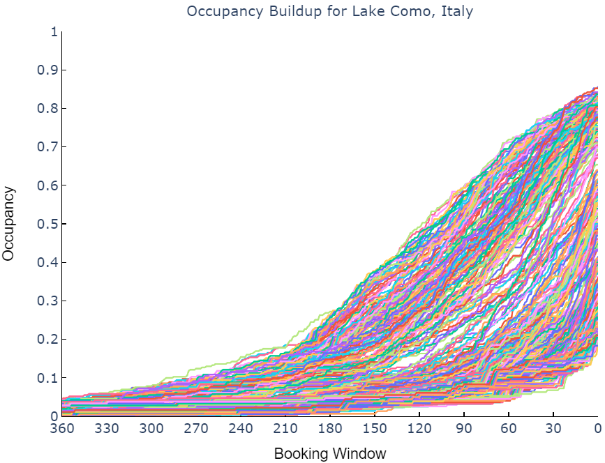
Let’s look at the image below that shows booking curves for Lake Como (Italy) – each line here represents the occupancy evolution for a date in the past. As you’d imagine, each date has a different booking curve.
The final occupancy of each date can be seen at the far right, where the occupancy ranges from 15% to 85%. Some dates show no occupancy 150 days out, while others start showing occupancy even as far as 300 days out. While each date has a different booking curve, some are “bunched” together, exhibiting similar booking patterns.
When forecasting demand for a date in the future “future date” (df), the first puzzle to solve is to find past “reference dates” (dr1,..,drk ) whose booking trends the future date is expected to follow. There are many options for selecting reference dates, such as:
- Same season
- Same day as week
- Holiday dates, or event dates,
- and even similarity scores calculated using the shape of the booking curve as of today.
This is a massive data science lift, especially at PriceLabs’ scale. This experimentation took us several months to find the right mix and the reference date. This is the science part of crystal ball forecasting!
We use the reference dates to understand how a future date is expected to book.
Many revenue managers get this part, though it is incredibly time-consuming. The exercise becomes easier, especially if you have prior year data for a listing or a market.
The next step is where continuous refinement of the forecast happens – the reactive part of what’s happening in the market. As the future date gets closer to the stay date, we use two fundamental revenue management metrics to adjust our forecast: Pacing and Pickup.
- Pacing represents the current occupancy of the future date compared to our reference dates at the same booking window. Think of this as “speed” – am I booking faster or slower than in the past?
- Pickup represents how fast (or slow) bookings are currently coming in. Think of this as “acceleration” – we might be pacing behind compared to the past, but recently, we are getting a lot of bookings, and we can surpass the past reference date occupancy soon.
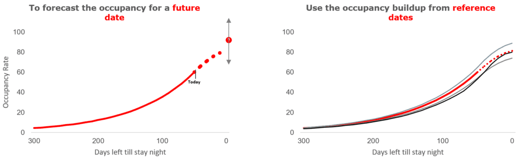
Mathematically, the forecast for a date is a function of our reference dates’ final booking curve and the future date’s booking curve till today. Many revenue managers look at the charts above manually daily to make an educated guess about the future.
Our algorithms do this at scale – daily, infallibly, and automatically. Instead of guessing, we measure what the function might look like for the forecast error to be low.

We process approximately 1 million data points every time we update rates a listing. We take immense pride in this as it involves extensive data engineering to do this in real time.
Unlock 4: Demand Elasticity
You likely know about elasticity from WSJ, Freakonomics podcast, or economics class.
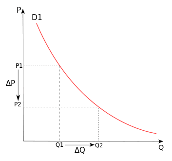
Economists use demand elasticity to measure the change in demand you can expect when you adjust the price up or down. It’s instrumental in production processes, for example – how many cars to produce. Cars, commodities, flight seats, etc., are generally available in large quantities, and demand generally means how many individual units can be sold.
But how do we understand how demand changes for vacation rentals with price? There is only one unique vacation rental – you can sell a night or not (100 % occupancy or 0% occupancy).
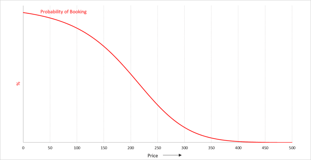
9 years ago, when we built our first algorithm, a literature survey led us to our first aha moment: instead of using “number of units expected to sell at a specific price” as demand, this problem required thinking of demand as “probability of getting booked” (PB) at different prices.
The probability of getting booked differs for each date for various price points; even for a given date, it changes over time. As the demand forecast changes, the probability of booking at a specific price changes.
We estimate market elasticity for each date in the future, as the underlying market factors like demand forecast, market prices, and demand sensitivity differ for each date. The market’s elasticity must be translated into your listing’s unique elasticity curve, determining your probability of booking at different prices.

The charts below show how elasticity can vary depending on the market sensitivity and demand forecast, both of which depend on how the market is evolving for a future date. The impact of market prices is absorbed in the scale on the x-axis.
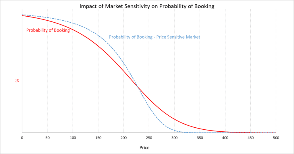
Probability of Booking as a Function of Market Sensitivity: The chart above shows two estimates of the probability of booking – the red one is identical to the first elasticity curve we showed above. In comparison, the blue curve represents a market that’s more sensitive to prices and, therefore, has a steeper slope at “normal” prices. Decreasing the price a little bit from the base price results in a much higher chance of booking, and increasing it a little bit greatly reduces it. We estimate the right price sensitivity for every hyper-local comp-set and future date. This is very evident in mountain markets, where the market is a lot less price sensitive in the Ski season than in the Summer season. However, the overall demand forecast is similar.
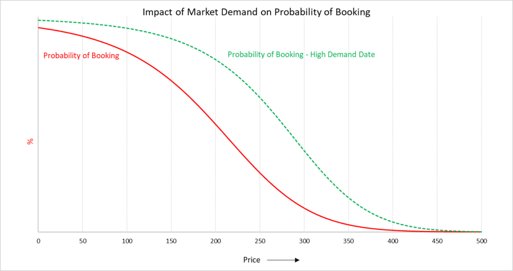
Probability of Booking as a Function of Demand Forecast: In this chart, the red line shows the probability of booking on a normal day, while the green curve shows the probability of booking on a high-demand date. Notice that the overall slope around the “normal” price is similar, but the entire curve is shifted to the right. This means that if you just hold your price steady on a high-demand date, the probability of getting significantly booked increases.
You’ll notice that at very low prices, the probability of booking doesn’t keep climbing up. In other words, even if the price is reduced to close to 0, it doesn’t guarantee a booking! This is because of multiple factors, but an important one is “perceived value.” Commodities (like oil) have globally acknowledged quality standards. Thus, very low prices result in very high demand.
But vacation homes don’t have a standard measure of quality. Guests book homes based on perceived quality and physical quality (photos and amenities). In such scenarios, price acts as a signal quality.
So, if you sell for very cheap, you may not sell every night (and would make a lot less – something we’ll see next!). These elasticity curves help us estimate how the market will react to price changes within your comp-set for every future date.
Unlock 5: Revenue Maximization
Once you understand the probability of a future date booking at a given price, the optimal price P’ is the price that maximizes the “expected revenue” (ER).
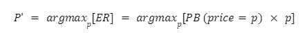
You can use the good old calculus book to differentiate the expected revenue function above or work through each possible price point and see which ones maximize your “expected revenue.”
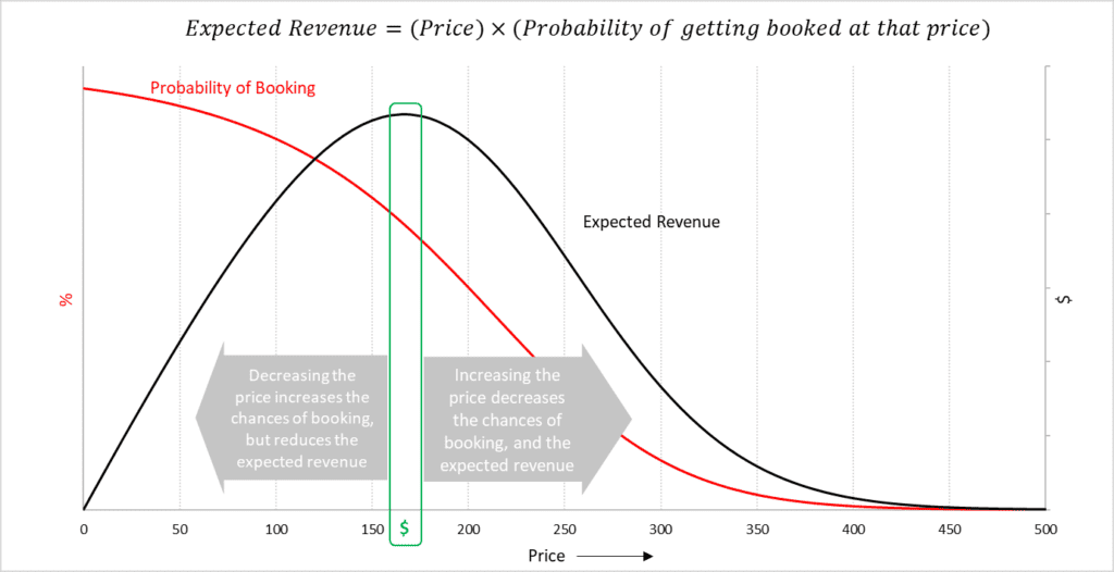
The chart above shows that at low price points, booking probability is high, but little to no money is made. On the other hand, at very high price points, booking probability is so low that we’ll not make any money again. The sweet spot is highlighted by the box where the expected revenue peaks.
In this first part of Dynamic Pricing Overview, we explored how PriceLabs calculates prices for any given day, one day at a time. The next challenge is how booking opportunities and, thus, rates will evolve. Say we are looking to price a date that is 365 days out, To optimize revenue, prices need to be updated daily for each of the 365 days in the future. This means that instead of finding a single optimal price, you need to determine a series of optimal prices over time, resulting in a sequence of price decisions.
This is a complex problem to solve. We use Dynamic Programming techniques to tackle the challenge of setting optimal prices over time, considering changing booking opportunities, frequent price adjustments, and the vast number of possible price combinations. We cover this in part 2 of this blog series.
If you’re ready to experience the benefits of dynamic pricing, we invite you to give PriceLabs a try – Start your Free Trial. Whether you’re a seasoned property manager or just starting out, our algorithm is designed to empower you.
If you have any questions about the above or PriceLabs in general please do reach out to our support team and they will loop us in!
Back to building,
PriceLabs Data Science Team