Updated: September 14, 2023
Unlock the Secrets of PriceLabs’ Cutting-Edge Dynamic Pricing Algorithm. Delve into the Depths – A Technical Adventure Awaits!
In Part 1 of our Dynamic Pricing Algorithm Overview, we reveal how we calculate optimal prices for any future date by forecasting its occupancy, estimating the probability of booking, and finding the price that maximizes the expected revenue.
The first part goes into why prices should be different by season, day of the week, how the market is pacing, and if there is a demand spike due to a holiday or event. If you have not read Part 1 yet, we recommend reading it before diving deeper into this article.
We now come to the last part of our algorithm: Rate Evolution, or how prices for a future date change over time. There are two main reasons why our price recommendations change over time.
Evolving forecast: Our forecast for a future date can change every day as we get new information. The chart below shows how our forecast for April 14, 2023 in the Phoenix market evolved in the preceding months. We see a sudden jump in the forecast after November 2022. Taylor Swift announced her Eras Tour dates for Phoenix, AZ. During August – October 2022, our market forecast had been reducing because the area were pacing behind previous year trends, picking up on the early signs of the slowing economy. But soon after the Eras Tour announcement, the pacing trend reversed, and our forecast jumped up by roughly 25%.
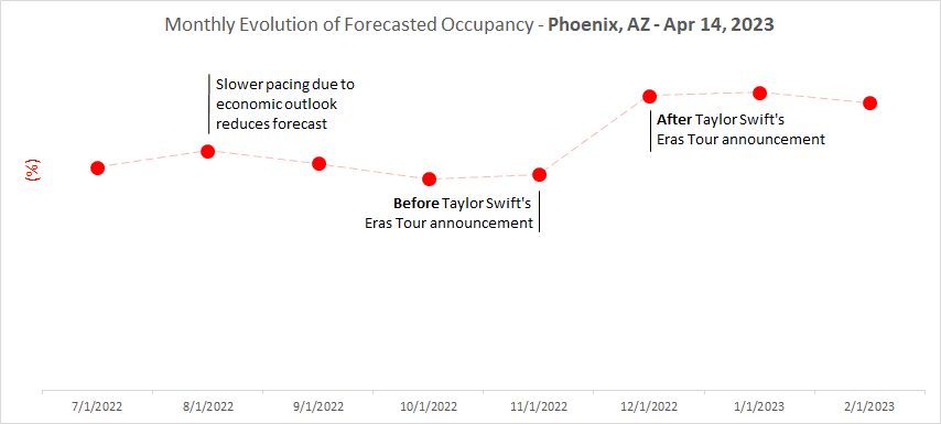
Note: The chart showing the monthly evolution of the forecast is for illustrative purposes only. The forecasting engine that powers wer dynamic pricing runs daily.
Remaining booking opportunity: In the example above, it is clear to anyone looking that as the forecast jumped up after the Eras tour dates were announced, the optimal prices should also jump up. But it is less clear how rates should evolve if our demand forecast for a date doesn’t change.
The upcoming sections help build the intuition around why and how the rates should evolve as we get closer to the stay date.
Why should prices change with lead time?
Our customers often ask us why our price recommendations are usually high for a far out date and reduced over time. We learned in the previous article that the probability of booking for a future date is tied to the forecasted occupancy.
For example, if the forecasted occupancy is 90%, and no bookings have happened. We expect 90 properties out of 100 similar properties to get booked. At that moment, we can pick a high price, given that most properties in the market are expected to be booked.
Let’s fast forward to 3 months out and say 80 properties are now booked. The market is pacing as expected, and we’re still forecasting 90% occupancy. This means that out of the remaining 20 properties, only 10 are expected to get booked – a 50% probability of booking.
While the overall market outlook hasn’t changed (we’re still expecting 90% occupancy), if wer property hasn’t been booked yet, the chances of it getting booked now while holding the same price have dropped. So, we might want to lower rates to increase expected revenue.
Unlock 7: Rate Evolution
Thus, we need to introduce “lead time” to the calculation of the probability of booking at different price points.
Let’s use another example to understand this better. Consider a scenario where:
- We can change prices 3 times at the following booking windows – 360, 240, and 120 days.
- Prices can be either 200, 400, 600, 800 or 1000.
- No one books more than 360 days in advance.
- The probabilities of booking at each booking window are in the table below.
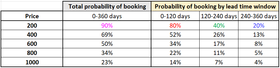
As we’ll notice – we now have access to what the probability of booking is in different booking windows. The total probability of booking at a price can be derived from the individual booking window probabilities.
For example, for a price of 200 -> the total probability of booking can be calculated using the formula below

Scenario 1: we can only set prices once
Let’s now calculate the maximum expected revenue in the two scenarios below.
In this case, the revenue maximizing price would be the one where the multiplication of the first two columns (price and the probability of booking at the price) is the highest. The price point of $600 provides the highest expected revenue of $300 ($600*50%). If we were only allowed to set a price once, $600 is what we’d go with!
Scenario 2: we can change the prices 3 times
Finding the optimal set of prices can be computationally challenging given the sequence of decisions with multiple possibilities and conditional probability. There are 5 possible prices for each of the three booking windows. That makes the total number of possibilities to explore 5*5*5 = 125 possibilities.
Now imagine if we had the same 5 and prices for the future date that is 360 days away. But now we can change the price daily. The number of possibilities now is 5^360. A very large number that’s difficult even for the fastest computers to solve!
The easiest decision to explain is the price 120 day booking window. At 120 days, the revenue-maximizing price can be calculated by multiplying the prices by the probability of getting booked 120 days out. In this case, 400 is the revenue-maximizing price for this window.
For 240 days booking window, we not only have to consider maximizing the revenue that can be made by selling in that window, but also the possibility of not selling and selling in the 0-120 day window. We don’t want to sell for too cheap now when we can possibly sell for $400 in the future. Optimizing this can be an involved exercise, but thankfully, this is a well-studied area of mathematical optimization. We solve this computation problem using the Bellman Equation.
We are providing an optimal solution to show that the expected revenue is more than what we’d find in Scenario 1.
The optimal set of prices below gives an expected revenue of $303:
- 360 days out: set to $800
- 240 days out: set to $600
- 120 days out: set to $400
Scenario 2 gives an expected revenue of $303 vs scenario 1 with an expected revenue of $300. Thus, scenario 2 performs 1% better.
While the above example showed a fairly modest 1% revenue gain from changing prices, our experiments with real data show the gains from correctly using last-minute discounts to be around 9%. The difference comes from the fact that our algorithms aren’t just changing prices 3 times a year, but doing it every day.
Note: we’ll notice that the price for the 0-120 day window has a discount on the optimal price from scenario 1, while the price for the 240-360 day window has a premium on the optimal price from scenario 1. Our algorithm automatically calculates these as lead time changes.
Increase prices at the last minute?
Yes! The above example assumes that our demand forecast is known at the beginning and doesn’t change. In reality, as we saw with the Taylor Swift Era’s concert, or economies slow down, a lot can happen as a date gets closer.
Prices can increase as a date gets closer if the market is booking up faster than our forecast. It can also happen when there is a significant difference in the price sensitivity of last-minute and early-bird bookings.
Why do Airlines do it differently?
While both Airlines and Vacation Rentals are a part of the travel industry, the market dynamics are very different.
Vacation rentals are close to “perfect competition” – for a potential guest, many options are available. In addition, the ownership of these options tends to be fairly fragmented – even in markets where a large manager manages most of the inventory, the revenue from a booking on one home isn’t shared with another homeowner.
Airlines are an oligopolistic market. There are only a few viable options on most routes from one city to another. Additionally, when we factor in last-minute business travel, three additional factors weigh in – loyalty programs that mean travelers are more likely to choose their preferred airline; enterprise sales contracts that mean large businesses exclusively book their employees on tends to their preferred airlines; and the generally lower price sensitivity of business travelers. All these mean that the revenue-maximizing decision for Airlines is frequently to keep prices higher at the last minute, even if that means a few empty seats. Unlike homes, the total revenue of the plane is what matters, not that each seat maximizes its revenue.
Far out premiums in vacation rentals serve another important function: when a date is very far out and the booking volume is low, there is an inherent margin for error in the forecast. We can do our best based on the data available, but lot of events can impact demand for a future date. Far out premiums serve as a hedge against such events, especially when the dates are far enough that not much of the demand was booking anyways.
Final note:
Setting prices to be dynamic for each future date is not a one-time exercise. Our data science team has found that even when the forecast is stable, the right far out premiums and last minute discounts give a 11% boost to revenue on average.
PS: We have some interesting insights on how the last-minute discounts should vary by market and by season – read this blog.
As we conclude our exploration of the dynamic pricing algorithm, we hope this article has shed light on the intricate process of optimizing your property’s rates. If you’re ready to experience the benefits of dynamic pricing, we invite you to give PriceLabs a try – Start your Free Trial. Whether you’re a seasoned property manager or just starting out, our algorithm is designed to empower you.
If you have any questions about the above or PriceLabs in general please do reach out to our support team and they will loop us in!
Back to building,
PriceLabs Data Science Team